Identifying Areas of Potential Aquaculture in the Western US
Author: William Mullins ・ Date: December 10, 2025
GitHubIntroduction
Does the suitable habitat area for oyster and blue mussel aquaculture differ across the western United States coast?
Oysters currently dominate mollusk aquaculture across the West Coast. According to the USDA 2023 Census of Aquaculture, mollusks account for 30% of all aquaculture sales in California, with oysters alone representing 26.6 percentage points—indicating that roughly 89% of California's mollusk aquaculture production is derived from oysters. Oregon and Washington show similar patterns of oyster dominance within their shellfish industries (USDA, 2024).
The relative lack of species diversification raises concerns about industry resilience. Region-wide stressors such as increasing ocean acidification or species-specific pathogens like Vibrio infections could simultaneously impact the majority of mollusk aquaculture facilities. The native blue mussel (Mytilus trossulus) represents a potential diversification candidate due to its different thermal tolerance nd established presence along the Pacific Coast.
This analysis investigates whether the current dominance of oysters is driven by environmental suitability by comparing suitable habitat areas for oysters versus blue mussels within the Exclusive Economic Zones of California, Oregon, and Washington. Suitable areas were classified by identifying locations where both sea surface temperature and depth fell within each species' tolerance range.
Datasets Used
- NOAA Pathfinder Sea Surface Temperature Data: Five-year average of sea surface temperature data from 2008-2012, providing a baseline for temperature analysis along the western US coast.
- NOAA Bathymetry Data: High-resolution ocean depth measurements used to identify suitable depths for shellfish cultivation.
- West Coast Regional Boundaries: Spatial boundaries defining the Exclusive Economic Zones (EEZs) for California, Oregon, and Washington, used to calculate suitable habitat area by region.
Loading Packages
Data Import
The following section imports the three datasets used in the analysis. We implement validation checks to ensure files exist before attempting to load them.
- The SST data are stored as individual GeoTIFF files, each representing the average annual SST for a given year. These rasters are stacked into a single multi-layer raster object.
- The bathymetry raster is then imported and reprojected to match the coordinate reference system of the SST stack.
- The EEZ boundaries are read as a vector layer.
Data Processing
To find the temporal mean SST across the 2008–2012 period, we compute the average across the raster stack. Since the original values are in Kelvin, we convert them to Celsius by subtracting 273.15.
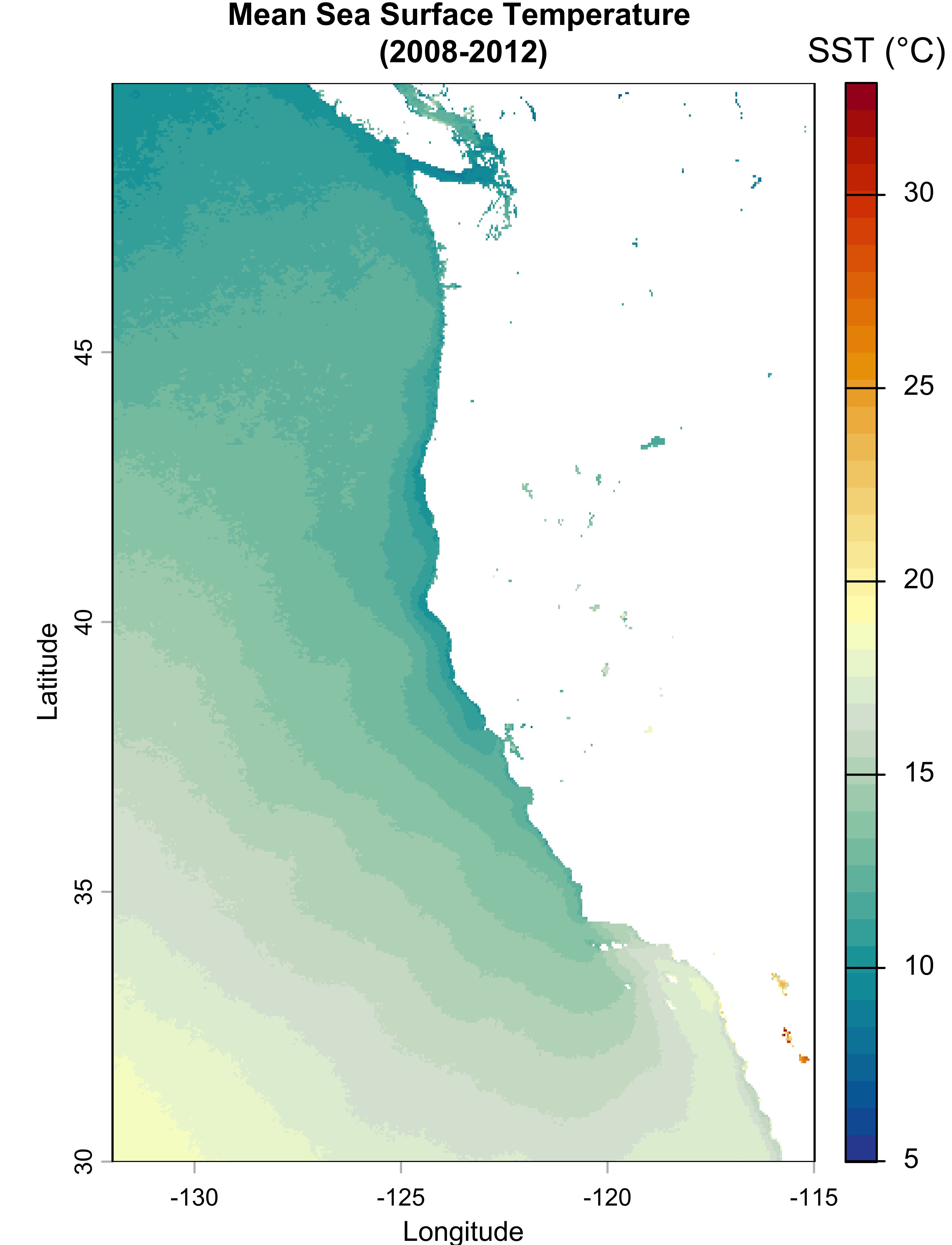
Interpretation: This map reveals the characteristic temperature gradient along the US West Coast. Southern California exhibits the warmest waters (20-25°C), while the Pacific Northwest and areas influenced by coastal upwelling show cooler temperatures (10-15°C). This spatial variation in temperature has important implications for species-specific aquaculture siting, as different shellfish species have distinct thermal tolerances.
Depth Data Preparation
The depth raster is resampled to match the resolution and extent of the SST data using nearest neighbor interpolation. This ensures that both datasets align perfectly for subsequent analysis.
Habitat Suitability Analysis
To evaluate the potential of locations for marine aquaculture of a given species, we use measurements of environmental tolerances. Using these thresholds, each pixel in the study area is classified as either suitable or unsuitable based on whether it simultaneously satisfies both temperature and depth criteria.
Suitability Function
The find_suitable_habitat() function implements this logic by first generating binary masks for temperature and depth suitability. The rasters are then combined, producing a categorical raster containing locations where both conditions are met.
Map of Potential Oyster Habitats
Oysters prefer slightly warm waters (11-30°C) and are able to be cultivated in shallow depths (0-70 meters).
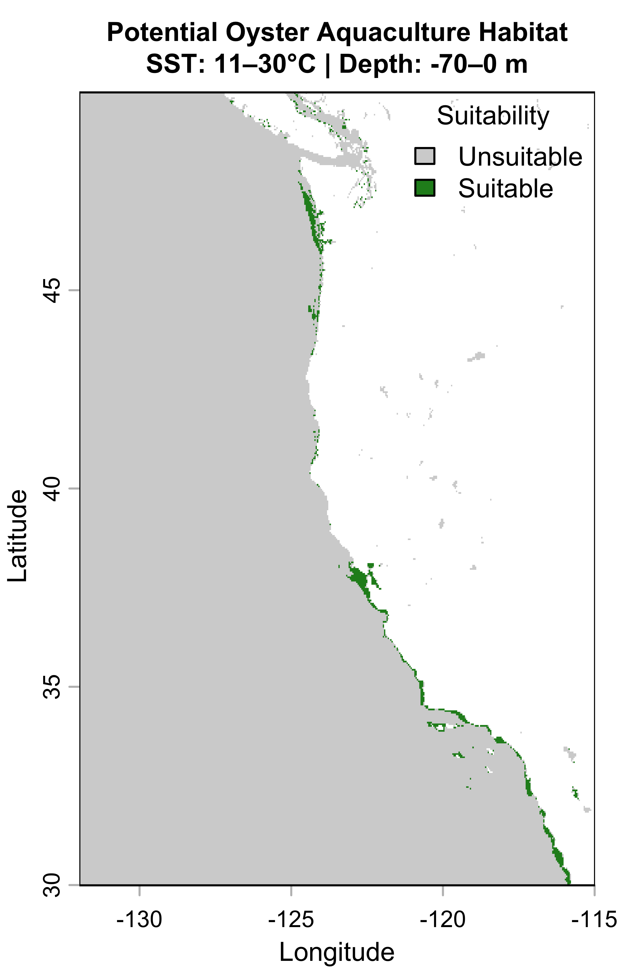
Interpretation: This map shows that suitable oyster habitat is concentrated along the coast of Southern and Central California, with a substantial area also present in Washington. The warmer waters of Southern California are particularly favorable, while Washington's extensive shallow coastal areas likely contribute to its suitability. Oregon and Northern California appear to have significantly smaller amounts of suitable area, likely due to cooler water temperatures from coastal upwelling.
Map of Potential Mussel Habitats
The species of blue mussels native to the West Coast, Mytilus trossulus, is cold-adapted (-1 to 20°C) and restricted to shallower depths (0-24m), which significantly limits suitable area compared to oysters. Washington's cooler waters and extensive shallow coastal zones in areas like Puget Sound likley make it the most favorable region.
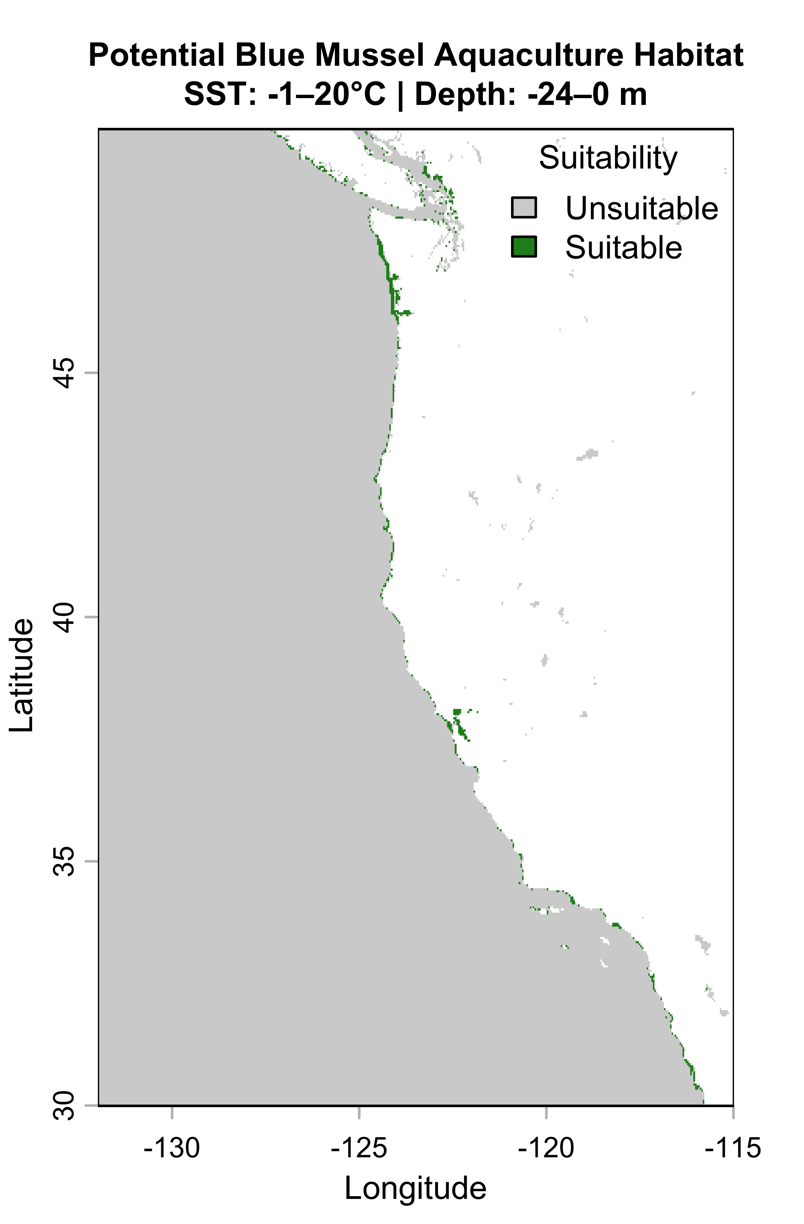
Interpretation: This map shows that suitable blue mussel habitat is primarily found within Washington, with a secondary cluster present in the San Francisco Bay area of Central California. Their preference for cooler and shallower waters is likely the cause of their smaller suitable area size in the south and central coast. Washington's cooler waters and extensive shallow coastal zones in areas like Puget Sound likley make it the most favorable region.
Regional Analysis of Suitable Habitat
To quantify aquaculture potential by jurisdiction, we calculate the total area of suitable habitat within each state's Exclusive Economic Zone.
Calculating Suitable Area by Region
This function builds upon the habitat suitability analysis by calculating the total area (in square kilometers) of suitable habitat within each region.
Table of Suitable Area by Region
| Region | Oysters (km²) | Blue Mussels (km²) |
|---|---|---|
| Central California | 4940.04 | 1533.94 |
| Northern California | 454.30 | 748.67 |
| Oregon | 1578.972 | 1181.82 |
| Southern California | 4221.39 | 1140.71 |
| Washington | 3313.16 | 2878.92 |
Table 1: Suitable Area For Oysters and Blue Mussels by Region
Interpretation
- Washington has the most suitable habitat for blue mussels (2,878.92 km²), which is almost double the amount of the next highest region. This is likely due to the cold waters of the state and extensive shallow areas found in regions like Puget Sound.
- Central California leads in oyster habitat suitability (4,940.04 km²), likely due to its warmer waters. This region shows a significant disparity between suitable oyster and mussel habitat (4,940 km² vs. 1,534 km²).
- Oregon shows a slight preference for oysters over mussels (1,578.97 km² vs. 1,181.82 km²), though conditions are relatively balanced for both species.
- Southern California shows high suitability for oysters (4,221.39 km²) with below-average suitability for mussels (1,140.71 km²), consistent with its warmer waters exceeding the mussel temperature tolerance.
- Northern California is the only region where mussel-suitable habitat (748.67 km²) exceeds oyster-suitable area (454.30 km²), likely due to cooler waters from coastal upwelling.
Implications for Aquaculture Development
The results of this analysis suggest that the current dominance of oyster aquaculture along the West Coast may not fully reflect the environmental potential for species diversification. The suitability analysis revealed that opportunities for blue mussel cultivation appear to remain largely untapped. Washington emerges as the most promising region for mussel diversification, with 2,879 km² of suitable habitat—more than double that of any other region. Northern California also presents a compelling case, as mussel-suitable habitat (749 km²) exceeds oyster-suitable area (454 km²), a pattern not reflected in current farming practices.
Central and Southern California's substantial oyster-suitable areas (4,940 km² and 4,221 km² respectively) support the industry's continued focus on oysters in these regions. However, it is worth noting that the majority of oyster farming is located in the northern half of the state, indicating that these southern regions may be generally underutilized for shellfish production. Oregon shows relatively balanced conditions for both species, with a slight advantage for oysters (1,579 km² vs. 1,182 km² for mussels).
These findings are significant when viewed through the lens of industry resilience. As noted in the introduction, approximately 89% of California's mollusk aquaculture production derives from oysters. This concentration leaves the industry vulnerable to the region-wide stressors identified earlier: increasing ocean acidification and species-specific pathogens. This analysis demonstrates that environmental conditions along the West Coast could support greater species diversification, particularly through expanded blue mussel cultivation in Washington and Northern California.
Limitations
While this analysis provides a solid foundation for further research, it has some limitations that should be addressed in future research:
- Temporal Resolution: The data uses annual SST, which does not account for seasonal variations in ocean conditions. Locations which experience extreme seasonal differences are likely to go undetected using this method, which could result in false positives being introduced.
- Environmental factors not considered: Important variables such as acidity, tidal patterns, wave exposure, and El Niño events were not included in the analysis.
- Socioeconomic and Regulatory Constraints: Shipping lanes, marine protected areas, and competing ocean uses were not incorporated into the suitability model.
Future Research
In addition to addressing the above limitations, future research should investigate the economic viability of establishing mussel production in areas identified as suitable. Additionally, climate forecasts should be included in the analysis to see if sites are likely to remain suitable in the future.
References
- National Oceanic and Atmospheric Administration. (2023). NOAA CoastWatch Pathfinder Sea Surface Temperature Dataset. https://podaac.jpl.nasa.gov/dataset/AVHRR_PATHFINDER_L3_V52
- National Centers for Environmental Information. (2023). Gridded Bathymetry Data. https://www.ncei.noaa.gov/access/gridded-bathymetry-data
- NOAA Fisheries. (2023). West Coast Regional Boundaries. https://www.fisheries.noaa.gov/west-coast/marine-protected-areas/west-coast-regional-boundaries
- Food and Agriculture Organization. (2022). The State of World Fisheries and Aquaculture. https://www.fao.org/3/ca9229en/ca9229en.pdf
- United States Department of Agriculture (USDA) National Agricultural Statistics Service. 2024. 2023 Census of Aquaculture. https://www.nass.usda.gov/Publications/AgCensus/2022/Online_Resources/Aquaculture/index.php