Regional Water Use Efficiency in California Vineyards
Author: William Mullins ・ Date: December 5, 2025
GitHubIntroduction
The California Water Challenge
Does hydrologic region affect vineyard water use in California, after controlling for evapotranspiration, precipitation, and irrigated crop area?
California's agriculture is the state's dominant water consumer, accounting for approximately 80% of its developed water supply. The efficiency of this water use is paramount for economic resilience and environmental stewardship, particularly as climate change exacerbates drought frequency and intensifies competition for limited resources.
Vineyards represent a significant and geographically diverse component of the state's agricultural portfolio, spanning disparate climate zones from the cool coastal valleys to the hot interior regions. While climatic factors are known drivers of water demand, regional differences inherent to California's 10 major hydrologic regions include additional variables such as such as water management practices, regulatory structures, soil characteristics, and crop varieties—may exert an independent and measurable influence on observed water use efficiency.
The aim of this analysis is to quantify the magnitude and direction of the independent effect of hydrologic region on vineyard water use efficiency across California.
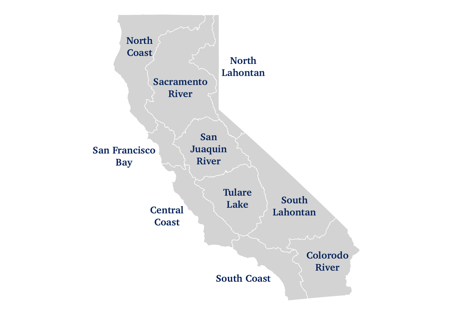
California Hydrologic Regions
The state is divided into 10 hydrologic regions, each with distinct climate characteristics that influence agricultural water demand.
About the Data
Data was extracted from the California Department of Water Resources Statewide Agricultural Water Use Data (2016-2020) Excel Application Tool. This dataset provides annual estimates for water use variables across 20 crop types and multiple geographic scales.
Key variables used in this analysis:
- Regional Applied Water Volume (AW): Total irrigation water applied to vineyards in acre-feet
- Regional Irrigated Crop Area (ICA): Total vineyard acreage receiving irrigation
- Regional Crop Evapotranspiration ($ET_c$): Total water lost to atmosphere from soil and plants (acre-feet)—represents crop water demand
- Regional Effective Precipitation ($E_p$): Rainfall that effectively contributes to crop water needs (acre-feet)
- Hydrologic Region (HR): California's 10 major hydrologic regions, defined by watershed boundaries and climate characteristics
Data availability: California DWR Water Use Data.
Directed Acyclic Graph (DAG)
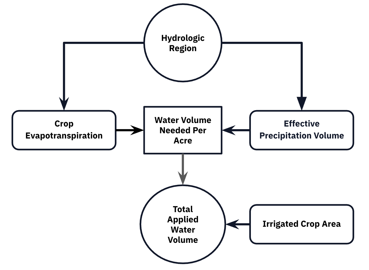
The following DAG illustrates the conceptual model of how the variables relate:
- Hydrologic Region (HR) → Climate Driven Variables: HR defines the local climate conditions. Different regions have different temperatures, humidity, and weather patterns. This drives both $ET_c$ (water lost) and $E_p$ (water gained naturally).
- Climate Driven Variables → Water Use: After accounting for natural water supply ($E_p$), the deficit between demand ($ET_c$) and supply must be met through irrigation.
- Vineyard Size (ICA) → Total Volume: Larger vineyards require proportionally more total water (a scaling relationship).
After controlling for climate and size, regional coefficients isolate potential management efficiency differences. The reference region (Central Coast) represents the efficiency baseline.
Import Packages
The analysis requires the following packages:
Data Processing Pipeline
The data is stored in an Excel application, which means that data for each of the variables is stored on its own individual sheets. The following code is used to read in data from each of the sheets and convert it into a standard data frame.
Data Preparation
Now that the data has been read in, we can select data collected from vineyards which applied water to their crops.
Data Exploration
Regional Water Use Summary
| Hydrologic Region | n | Mean AW | Median AW | SD | SE |
|---|---|---|---|---|---|
| South Lahontan | 23 | 128.78 | 39.43 | 295.28 | 61.57 |
| South Coast | 46 | 1,287.72 | 296.49 | 2,120.16 | 312.60 |
| Sacramento River | 206 | 3,631.83 | 134.91 | 8,249.17 | 574.75 |
| North Coast | 121 | 5,936.57 | 443.85 | 10,137.34 | 921.58 |
| Colorado River | 25 | 6,748.80 | 386.15 | 13,446.13 | 2,689.23 |
| Central Coast | 163 | 9,917.94 | 1,476.95 | 22,978.53 | 1,799.82 |
| San Francisco Bay | 80 | 10,135.80 | 138.55 | 25,803.39 | 2,884.91 |
| San Joaquin River | 182 | 17,764.87 | 3,262.99 | 41,878.19 | 3,104.22 |
| Tulare Lake | 166 | 38,072.24 | 5,663.51 | 58,246.36 | 4,520.79 |
Applied Water (AW) summary statistics by Hydrologic Region
Key observations:
- Large variation between regions: Mean water use ranges from 129 acre-feet (South Lahontan) to 38,072 acre-feet (Tulare Lake)—a nearly 300-fold difference
- High within-region variability: Standard deviations exceed means in all regions, indicating right-skewed distributions
- Median < Mean everywhere: Consistent with right skew caused by a few very large vineyard operations
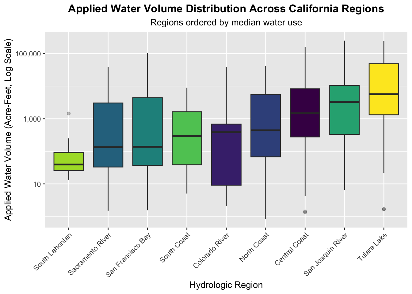
Distribution of Water Use
This log-scale boxplot reveals that while most regions have modest median use (100-1,000 acre-feet), there are many high water volume outliers in regions like Central Coast, San Joaquin River, and Tulare Lake.
Statistical Model
Model Specification
Why Gamma?
The Gamma distribution is appropriate here because:
- Positive support: Water use cannot be zero or negative in irrigated areas
- Right-skewed: The distribution has a long right tail (high outliers)
- Mean-variance relationship: Variance increases with the mean (heteroscedasticity)
Model Statistical Notation
Where:
- $Y_i$ = Regional Applied Water Volume for observation $i$
- $k = 1/\phi$ is the shape parameter (constant across observations)
- $\phi$ is the dispersion parameter
- $\theta_i$ is the scale parameter (varies by observation)
Gamma Regression Equation:
Coefficient Interpretation:
- $\beta_1, \beta_2$: Multiplicative change in water use per unit increase in $ET_c$ or $E_p$
- $\beta_3$: Change in water use per % change in vineyard area
- $\beta_4 - \beta_{11}$: Regional multiplier relative to Central Coast (reference region)
Model Fitting
| Parameter | Estimate | Std. Error | t value | Pr(>|t|) |
|---|---|---|---|---|
| (Intercept) | 7.473e-01 | 1.753e-02 | 42.624 | < 2e-16 *** |
| Regional_ETc_Vol | 9.758e-07 | 3.035e-07 | 3.215 | 0.00135 ** |
| Regional_Ep_Vol | -7.294e-06 | 2.672e-06 | -2.730 | 0.00645 ** |
| log(Regional_ICA) | 1.010e+00 | 2.213e-03 | 456.617 | < 2e-16 *** |
| HRColorado River | 6.531e-01 | 3.313e-02 | 19.712 | < 2e-16 *** |
| HRNorth Coast | -1.257e-02 | 1.857e-02 | -0.677 | 0.49850 |
| HRSacramento River | 2.045e-01 | 1.645e-02 | 12.432 | < 2e-16 *** |
| HRSan Francisco Bay | 5.207e-02 | 2.117e-02 | 2.460 | 0.01406 * |
| HRSan Joaquin River | 2.495e-01 | 1.660e-02 | 15.029 | < 2e-16 *** |
| HRSouth Coast | 3.332e-01 | 2.572e-02 | 12.956 | < 2e-16 *** |
| HRSouth Lahontan | 5.557e-01 | 3.475e-02 | 15.993 | < 2e-16 *** |
| HRTulare Lake | 5.399e-01 | 1.755e-02 | 30.769 | < 2e-16 *** |
Gamma GLM Coefficient Estimates (Dispersion parameter: 0.0234)
Signif. codes: 0 '***' 0.001 '**' 0.01 '*' 0.05 '.' 0.1 ' ' 1
Model Validation Through Simulation
To ensure the model is correctly specified and is able to reliably estimate parameters, simulations are used. This process involves:
- Using coefficients from the model as the "true" values
- Generating 500 synthetic datasets using those parameters
- Refitting the model for each dataset
- Checking if that model recovers the true parameters
Simulation Procedure
Simulation Results
| Parameter | True Value | Recovered | Difference | % Error |
|---|---|---|---|---|
| (Intercept) | 7.473e-01 | 7.427e-01 | 4.60e-03 | 0.62 |
| Regional_ETc_Vol | 9.758e-07 | 8.633e-07 | 1.12e-07 | 11.52 |
| Regional_Ep_Vol | -7.294e-06 | -8.424e-06 | 1.13e-06 | 15.49 |
| log(Regional_ICA) | 1.010e+00 | 1.010e+00 | 3.76e-04 | 0.04 |
| HRColorado River | 6.531e-01 | 6.622e-01 | -9.14e-03 | 1.40 |
| HRNorth Coast | -1.257e-02 | -5.219e-03 | -7.35e-03 | 58.49 |
| HRSacramento River | 2.045e-01 | 1.988e-01 | 5.74e-03 | 2.80 |
| HRSan Francisco Bay | 5.207e-02 | 3.966e-02 | 1.24e-02 | 23.84 |
| HRSan Joaquin River | 2.495e-01 | 2.610e-01 | -1.15e-02 | 4.62 |
| HRSouth Coast | 3.332e-01 | 3.452e-01 | -1.20e-02 | 3.59 |
| HRSouth Lahontan | 5.557e-01 | 5.573e-01 | -1.54e-03 | 0.28 |
| HRTulare Lake | 5.399e-01 | 5.557e-01 | -1.58e-02 | 2.93 |
Parameter Recovery Summary (Mean absolute % error: 10.47, Max: 58.49)
Interpretation: For all of the parameters the model was able to recover the true value of the mean within its 95% confidence interval. This suggests that the model is successfully able to recover the parameter values.
Statistical Inference
Hypothesis Testing
Overall Test: Do Regions Differ?
Null Hypothesis ($H_0$):
All HR coefficients are zero, meaning there are NO differences in water use between hydrologic regions after controlling for climate factors and vineyard size.
Alternative Hypothesis ($H_1$):
At least one region differs in water use, indicating that regional factors beyond climate (e.g., efficiency, technology, regulations) affect water use.
Likelihood Ratio Test
The $H_0$ is tested by comparing the full gamma model (with HR) to a reduced gamma model (without HR):
| Model | Resid. Df | Resid. Dev | Df | Deviance | Pr(>Chi) |
|---|---|---|---|---|---|
| Null (without HR) | 1008 | 63.545 | - | - | - |
| Full (with HR) | 1000 | 23.979 | 8 | 39.566 | < 2.2e-16 *** |
Analysis of Deviance Table (Likelihood Ratio Test)
Results:
- Test Statistic: $\chi^2$ = 39.57 (df = 8)
- P-value: < 2.2e-16
- Conclusion: We reject the null hypothesis. There is evidence that the hydrologic regions affect the water applied by vineyards even after controlling for climate demand, precipitation, and vineyard size.
Individual Region Comparisons
Percent Change Calculation
Visualizing Regional Coefficients
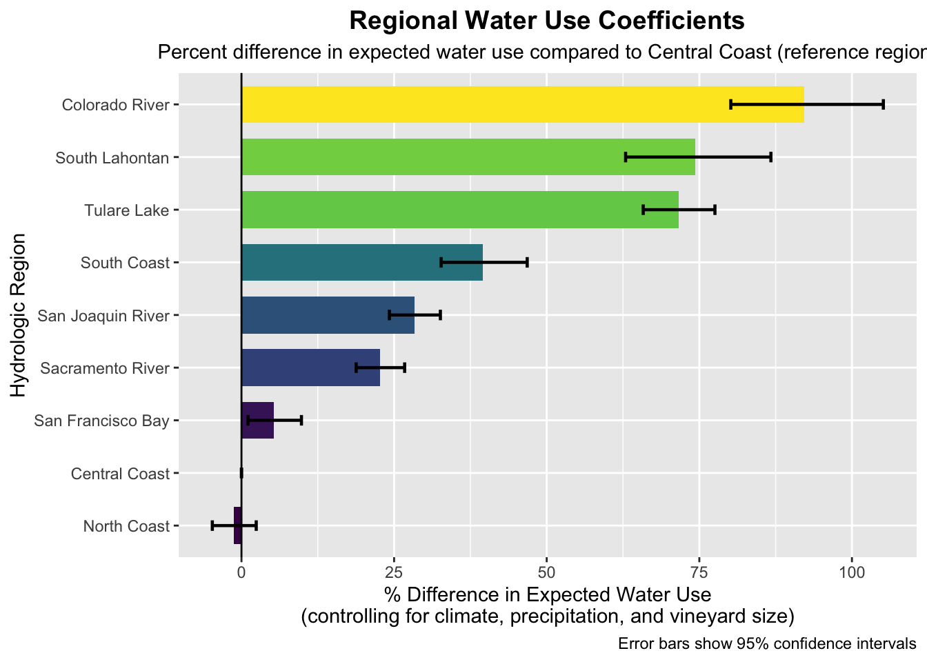
Of the nine regions, only one, the North Coast, did not differ a statistically significant amount from the coefficient of the Central Coast.
Model Fit and Diagnostics
Predicted vs Observed Values
Model Validation Metric
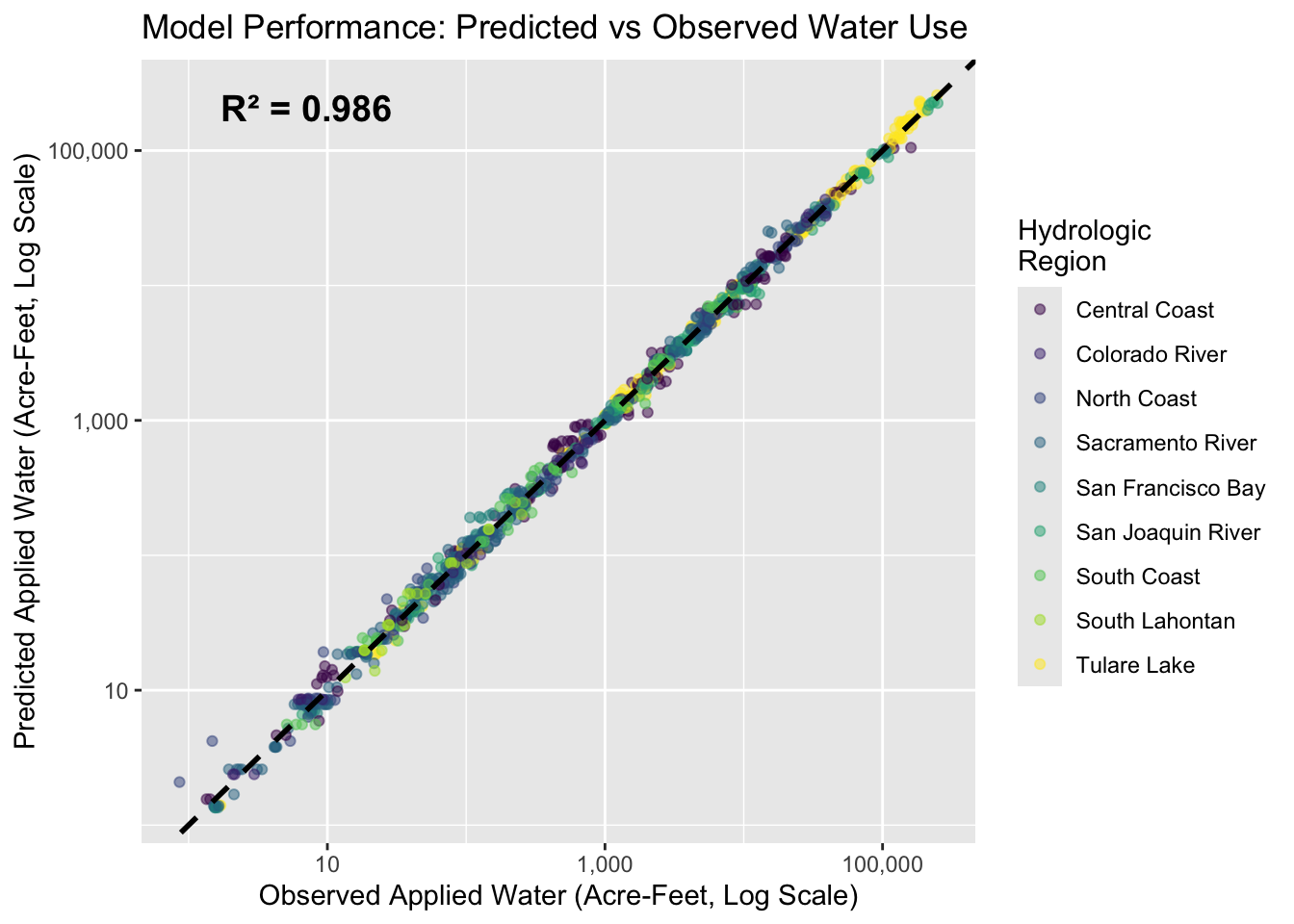
The model explains 98.6% of variance in water use, indicating excellent fit.
Discussion
Key Findings
This analysis provides evidence that hydrologic regions in California differ substantially in vineyard water use efficiency even after accounting for climate-driven water demand, effective precipitation, and vineyard size.
Main Results
- Regional effects are statistically significant and large
- LRT test: $\chi^2$ = 39.6, p < 0.001
- Coefficients ranged from -1% to +92% percent different from reference level
- Three regions show substantially higher coefficients
- Colorado River: 92% higher expected water use
- Tulare Lake: 72% higher expected water use
- South Lahontan: 74% higher expected water use
- Model validation confirms reliability
- Simulation showed parameter recovery
- High $R^2$ (0.986) — the majority of variation can be explained by the model
Future Directions
Further investigation should be done into finding what is causing the regional variation in water use between the regions. The results of this investigation imply that additional variables outside of water need are affecting some of these regions. Investigations should look into whether this is caused by management decisions or by additional environmental factors not considered in this study.